An image of a calculator and coins.
Tax Multiplier Formula
Definition
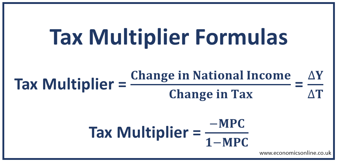
In economics, tax multiplier is defined as the ratio between change in national income (∆Y) and change in tax (∆T). The value of the tax multiplier is negative because any increase in tax by the government will affect national income negatively. Tax multiplier is a tool used by the governments so that they can reduce the tax rates by the exact amount that they want to raise the GDP. It allows governments to drive a precise change in taxes instead of estimation.
Tax Multiplier Formula
There are many formulas to calculate tax multiplier.

The first formula is:
Tax Multiplier = ∆Y/∆T
Here,
∆Y = Change in national income
∆T = Change in tax
The second formula is:
Tax Multiplier = -MPC/ (1-MPC)
Here
MPC = Marginal propensity to consume
Another formula is
Tax Multiplier = -MPC/MPS
Here
MPS = Marginal propensity to save
The negative sign in the formula indicates the decrease in taxes will promote spending and there will be an increase in national income.
Marginal Propensity to Consume
The amount a consumer or household will spend from each additional $1 added to their disposable income is called the marginal propensity to consume. It measures the fraction of additional income that households consume.
Marginal Propensity to Save
The amount a consumer or household will save from each additional $1 added to their disposable income is called marginal propensity to save.
Both marginal propensities to consume and save will always equal 1 when we add them. Any amount that consumers do not save will automatically be spent per $1, and vice versa. Hence, both MPS and MPC must be equal to 1 when added together, as consumers can only spend or save a portion of $1.
Derivation of Tax Multiplier Formula
Let’s understand the derivation of the formula of tax multiplier for the three-sector economy, with household sector, firm sector, and government sector.
In three-sector closed economy,
Y = C + I + G --- (1)
Here,
Y = National income
C = Consumption
I = Investment
G = Government spending
In Keynesian theory of income and employment determination,
C = C0 + MPC (Yd) is the equation of the consumption function.
Here,
C0 = Autonomous consumption
Yd = Disposable income = Y - T
So the consumption function becomes
C = C0 + MPC(Y-T)
Investment and government spending are autonomous, so
I = I0
G = G0
Putting all the values in the national income equation (1),
Y = C0 + MPC(Y-T) + I0 + G0
Y = C0 + I0 + G0+ MPC(Y-T)
∆Y = ∆ [C0 + I0 + G0+ MPC(Y-T)]
∆Y = ∆ (C0 + I0 + G0) + ∆ MPC(Y-T)
Since C0, I0, and G0 are all autonomous, so ∆ (C0 + I0 + G0) = 0
∆Y = 0 + ∆ MPC(Y-T) = ∆ MPC(Y-T) = MPC (∆Y) - MPC (∆T)
∆Y - MPC (∆Y) = - MPC (∆T)
∆Y (1 – MPC) = - MPC (∆T)
∆Y / ∆T = - MPC / (1 – MPC)
Tax Multiplier Example
Suppose that the value of MPC is 0.9, which means that consumers will spend 90 cents from every extra $1 income. Now let’s calculate the value of the tax multiplier.
Tax Multiplier = -MPC/ (1-MPC) = -0.9 / (1-0.9) = -0.9 / 0.1 = -9
This means that any decrease in tax by the government will increase gross domestic product or national income by 9 times and vice versa.
The Values of Tax Multiplier
The value of the tax multiplier varies from 0 to -∞. If the value of MPC is zero, which means that all of the income is saved by the households, the tax multiplier will be zero. If the value of MPC is 1, which means that all of the income is consumed by the households, the value of the tax multiplier will be -∞. 0 and -∞ are extreme values, and normally, the value lies between these two extremes.
The Strength of Tax Multiplier
The strength of the tax multiplier depends on the value of MPC. A higher MPC means a strong tax multiplier, while a lower MPC means a weak tax multiplier.
For example, if the value of MPC is 0.1, the tax multiplier will be -0.11, indicating a weak multiplier. On the other hand, if the value of MPC is 0.95, the tax multiplier will be -19, which indicates a strong multiplier.
Relationship between Tax and Spending Multiplier
Let’s now calculate the government spending multiplier by using the same value of MPC (0.9) as used in the above calculation example.
Government spending multiplier = 1/(1-MPC) = 1/(1-0.9) = 1/0.1 = 10
This means that any increase in government spending will increase the level of income by 10 times and vice versa.
The tax multiplier will raise the aggregate demand by a smaller amount as compared to the spending multiplier because when the government spends money, this means that the government will spend the exact amount of money that is already agreed upon, for example, $200 billion. In comparison, a tax cut or tax reduction will motivate people to consume only a portion of the tax cut while they conserve the rest. This will always result in a tax cut being weaker as compared to the spending multiplier.
Tax Multiplier Effect
The normal multiplier effect is that a small increase in investment, government spending, or exports will bring a large increase in national income and vice versa. However, due to the negative value, the tax multiplier effect is that a small decrease in tax will bring a large increase in national income and vice versa. This is due to the fact that consumer spending and taxes are inversely related to each other. An increase in taxes will decrease consumption. Hence, governments need to understand what the current condition of the overall economy is before changing any taxes. During recessionary periods, there are lower tax rates, but in inflationary periods, the tax rates rise.
Graphs
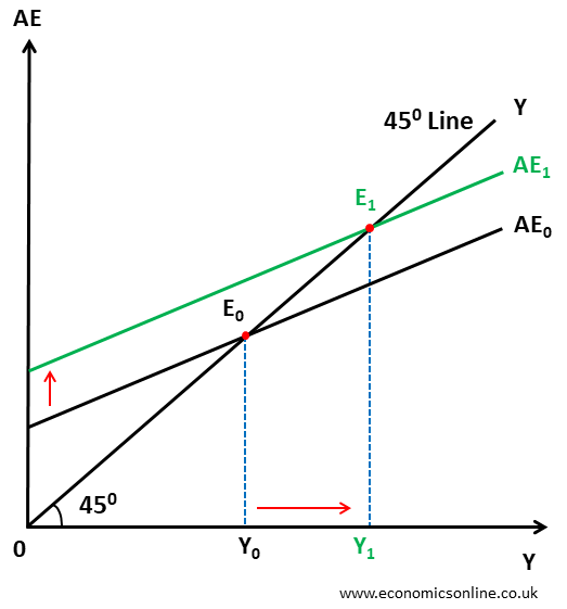
Let’s understand the tax multiplier with the help of graphs. The following graph illustrates the income-expenditure approach.

In this graph, national income (Y) is taken on the horizontal axis (x-axis) and aggregate expenditure (AE) is taken on the vertical axis (y-axis). The initial equilibrium point is E0, where the AE curve intersects the 45-degree line representing income. When the government reduces tax, the aggregate expenditure increases, and the AE curve is shifted upwards, leading to a new equilibrium point at E1 and an increase in national income to Y1.
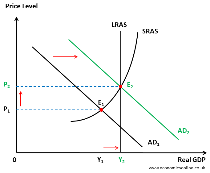
Let’s now use the AD-AS approach to illustrate the effect on the tax multiplier.

In this diagram, we have real GDP (the nation's economic output) on the x-axis and price level on the y-axis. At points P1 and Y1, the economy is in recession. A tax reduction will encourage consumers to spend more of their money since less of its portion is deducted in the form of taxes. This practice will lead to increased aggregate demand and allow the economy to attain equilibrium points at points P2 and Y2. At this point, both short-run and long-run aggregate supply curves are equal to the aggregate demand AD2.
How Taxes Alter GDP
If a rise in government spending leads to an increase in total GDP and spending, then a rise in taxes must lead to a reduction in total GDP and spending, and contrariwise. When the government increases taxes, then consumption reduces. Therefore, John Maynard Keynes distinguished that the reduction in overall spending from a tax increase is not as much as the overall increase in spending from the exact same amount of a government spending rise. The reason behind this is that people prefer to save a part of their additional income while the government consumes all of its money.
Conclusion
In conclusion, the tax multiplier evaluates the change in tax rates on overall economic output, particularly the change in aggregate demand due to the change in taxes. Tax multiplier is generally connected to a fiscal policy as it indicates how adjustments in taxes can trigger or shrink the economic activity of a country. The understandings of tax multipliers are critical for evaluating the impact of tax policies in affecting consumer spending and the overall economic health of a country.


