Image showing a developed city.
Long Run Aggregate Supply
The long-run aggregate supply (LRAS) curve depicts the relationship between the price level and the real GDP when there has been time for input prices to adjust to fluctuations in aggregate demand.
There are two types of long-run aggregative supply curves.
- The Keynesian LRAS
- The Classical LRAS
Keynesians: Supporters of the economist John Maynard Keynes who believe that the government intervention is necessary for an economy to reach at the full employment level.
Classical Economists: The economists who believe that the LRAS curve is vertical and that the economy will reach at the full employment level without government intervention.
1. The Keynesian LRAS
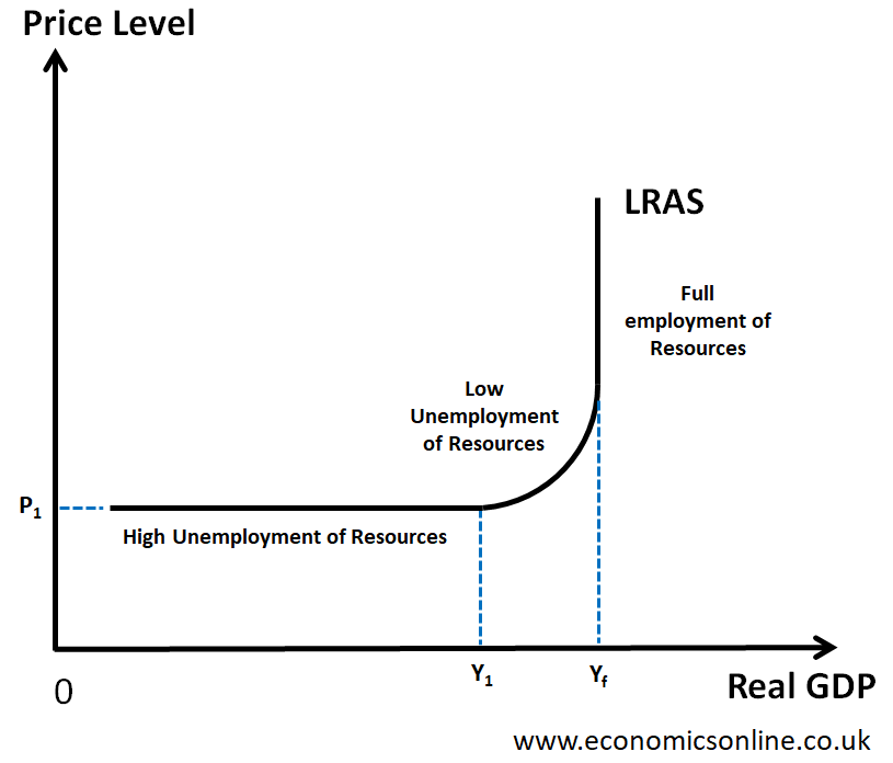
Keynesians represent the long-run aggregate supply curve as perfectly elastic at low output, then upward sloping over a range of output and finally perfectly inelastic at the full employment level of output. This is to emphasise their point that, in the long run, an economy can operate at any output level and not necessarily at the full employment level.

In the diagram, the LRAS is perfectly elastic (horizontal) if the economy has high unemployment of resources (before Y1). More output can be produced without an increase in costs of production and the price level, P1. At low output, firms can attract more resources without bidding up their prices. For example, at high unemployment, only the job offer may be enough to attract new workers.
The LRAS becomes more inelastic (upward sloping) as the economy approaches full employment ouput, between Y1 and Yf. The upward slope shows that the firms begin to face shortages of inputs and bid up wages, raw material prices and the price of capital equipment. Costs of firms will increase and, as a result, the price level will also increase.
The LRAS becomes perfectly inelastic (vertical) at Yf which is the full employment output (potential output), since at this point a further increase in the output is not possible. At Yf the economy is producing the maximum output it can make with the existing resources. This can also be shown by the points on the production possibility curve (PPC).
2. The Classical LRAS
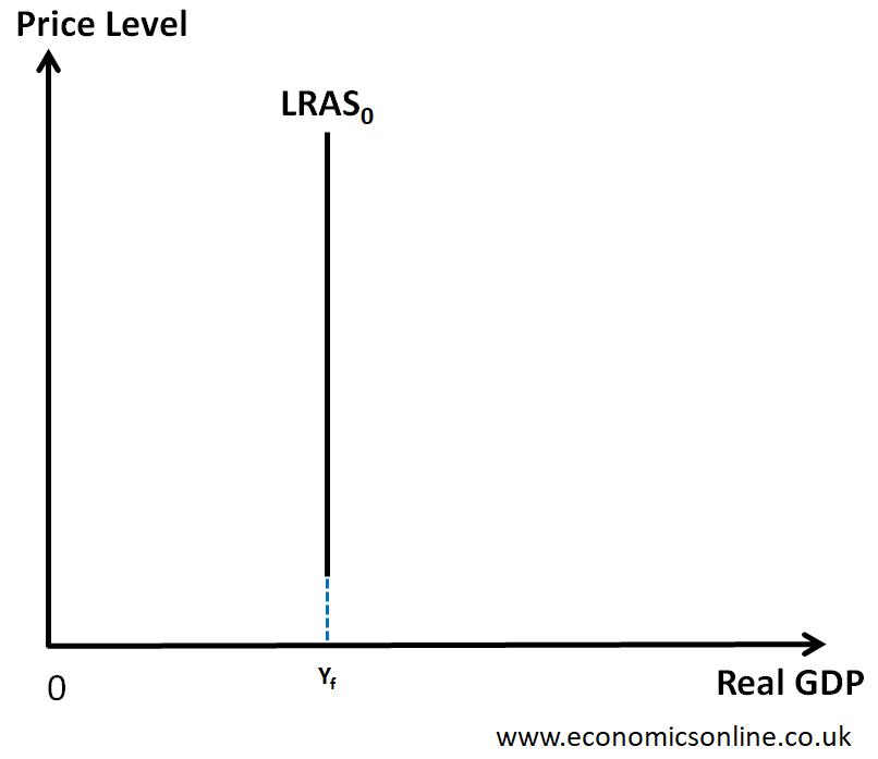
The classical economists believe that the LRAS curve is a vertical line at the full employment level of resources. This is because they think that in the long run the economy will operate at the full employment level of resources. This version of the LRAS curve is shown below.

In the diagram, the vertical LRAS shows that any change in the general price level will not affect the real GDP at all. Whether the price level rises or falls, the real GDP remains the same since the economy operates at the full employment of resources, that is, at Yf.
Another way to consider why the LRAS curve is vertical is to consider how real output responds to the changes in aggregate demand.
In the short run, and operating with spare capacity in the economy with an ‘output gap’, an increase in the aggregate demand can facilitate an expansion of aggregate supply, which means that the short-run aggregate supply curve (SRAS curve) is upward sloping.
However, in the long run, and assuming that all the factors of production are fully employed, any increase in the aggregate demand cannot induce more output – rather, the effect is on the price level and not on the real GDP.
Determinants of LRAS

Long-run aggregate supply curve shifts to the right or left due to the following reasons.
1. Changes in the Quantity of Resources
The first reason for the shift of the LRAS curve is the change in the quantity of resources in the economy. The quantity of resources available in an economy may change over the period of time leading to the shift of the LRAS.
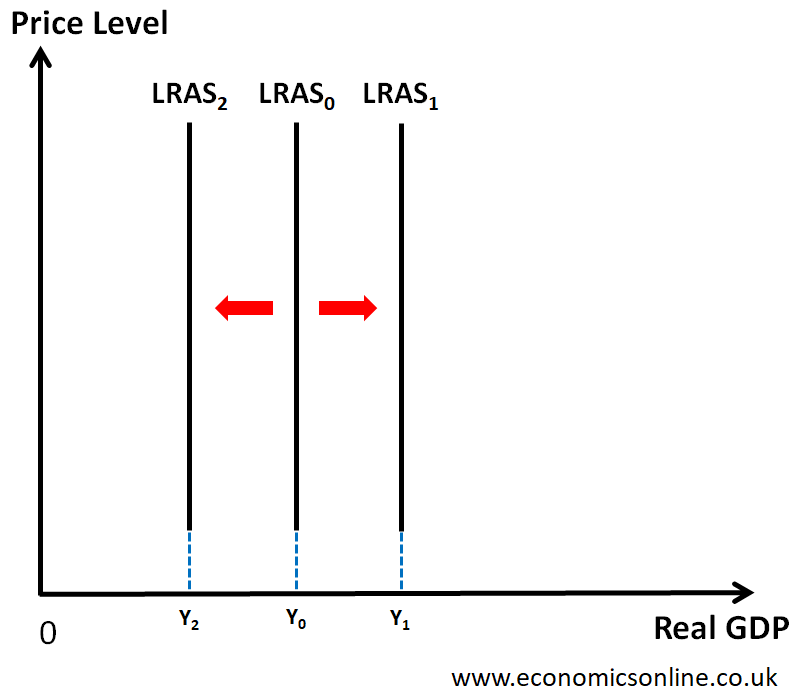
An increase in the quantity of resources will shift the LRAS towards right from LRAS0 to LRAS1. The quantity of land may be increased if new natural resources are discovered. The quantity of labour may be increased with an increase in the labour force due to increase in population, higher women participation or immigration. Similarly the quantity of capital may be increased by producing more capital goods or by importing them.
A decrease in the quantity of resources will shift the LRAS towards left from LRAS0 to LRAS2.
The quantity of land may be decreased if natural resources are depleted. The quantity of labour may be decreased with a decrease in the labour force due to the decrease in population or emigration. Similarly the quantity of capital may be decreased due to depreciation of capital goods which are not replaced.
2. Changes in the Quality of Resources
Another reason for the shift of the LRAS curve is the change in the quality of resources in the economy. The quality of resources available in an economy may change over the period of time leading to the shift of LRAS.
An increase in the quality of resources will shift the LRAS towards right from LRAS0 to LRAS1. The quality of land may be increased if the fertility of land is increased. The quality of labour may be increased with improvement in labour productivity due to better education and training. Similarly the quality of capital may be increased due to an improvement in technology.
A decrease in the quality of resources will shift the LRAS towards left from LRAS0 to LRAS2.
The quality of land may be decreased with a decrease in the fertility of land. The quality of labour may be decreased with a decrease labour productivity due to lower motivation, poor education and lack of training. Similarly the quality of capital may be decreased if machines become obsolete.
3. Changes in the Costs of Production
The final reason for the shift of the LRAS curve is the change in the costs of production over the period of time.
A decrease in the cost of production will shift the LRAS towards right from LRAS0 to LRAS1. On the other hand, an increase in the cost of production will shift the LRAS towards left from LRAS0 to LRAS2.


