
Photo by Simon Maage / Unsplash
Cobweb Theory in Economics
Introduction
In the market for agricultural products, prices fluctuate periodically. It means that a low price in one year is followed by a high price in the next year and then again a low price in the following year. This form of price oscillations cause market failure and can be explained with the help of the cobweb theory.
Cobweb Theory
Price fluctuations can cause a fluctuation in supply, which creates a cycle of rising and falling prices. This is referred to as the cobweb theory, cobweb theorem, cobweb cycle or cobweb model. The cobweb theory explains the price oscillations or fluctuations in agricultural markets and their endogenous dynamics. In one season, the price is high and in the next season, it is low. Then it is high again and then it is low again and this pattern continues. This is bad news for farmers. These price fluctuations make it difficult for farmers to make right investment decisions when harvesting their crops. They become clueless in deciding the supply of agricultural products from one year to the next.
Historical Background
The concept of the cobweb theory was first introduced by Professor Nicholas Kaldor in 1934. In 1930s, three other economists of the twentieth century also worked on this theory. Those three economists are Henery Schultz from the U.S.A., Jam Tinbergen from the Netherlands and Althus Hanau from Italy. This theory is called cobweb theory because the diagram of this theory resembles with the cobweb.
Assumptions of Cobweb Theory
The following are some assumptions of cobweb theory:
Supply Decision
It is assumed that in an agriculture market, farmers make supply decision based on the price of the agricultural commodity in the last year. When their own supply hits the market, they don’t know what will be the market price.
Main Determinant of Supply
It is also assumed that the last year’s price of the agricultural product is the main determinant of the supply.
Impact of Prices
It is assumed that a high price will attract more farmers to enter the market and grow agricultural products, while a low price will make some farmers leave the market.
Cobweb Diagram
In economics, the cobweb diagram illustrates the price fluctuation occurring in the market due to the quantity supplied by manufacturers, which totally depends on the prices in the last production period. For example, if wheat prices are high in the current year, the farmers prefer to harvest wheat in the next year in order to take advantage of the high prices, but as the supply increases due to high production, the prices will fall. Let’s illustrate the cobweb theory with the help of the following diagram:
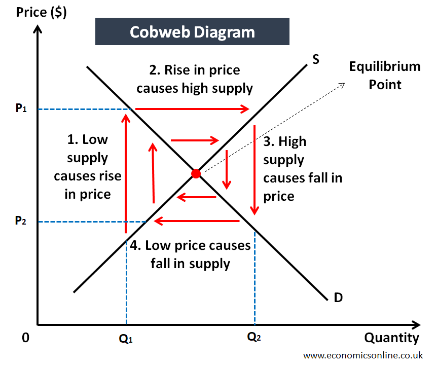
In the above diagram, quantity is on the horizontal axis (x-axis) and price is on the vertical axis (y-axis). The market is operating at equilibrium point where the demand curve D and the supply curve S intersect.
Suppose that, due to bad weather, the quantity supplied is at Q1. At Q1, buyers are willing to pay a higher price of P1 and sellers get benefit of that.
Due to this high price of P1 this year, next year farmers will increase supply. This high supply will reduce the price to P2.
This low price P2 will cause the supply to fall in the coming year. A low supply will cause the price to rise and so on. These continuous fluctuations will occur in the form of endogenous cycles. When farmers increase supply, they face a low price and when they decrease supply, they face a high price. This is how prices fluctuate, according to the cobweb theory.
Types of Cobweb Diagrams
The following are the types of cobweb diagrams based on convergent fluctuation and divergent fluctuation in prices:
Convergent Cobweb
The first type of the cobweb is the convergent cobweb in which price converges towards equilibrium price. In a convergent cobweb, the price elasticity of demand is more as compared to the supply, and the price volatility is decreasing. This is illustrated in the following diagram:
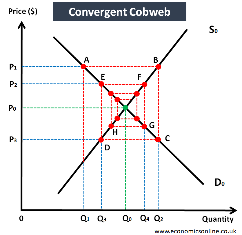
In the above diagram, the market is operating at equilibrium point where the demand curve D0 and the supply curve So are intersecting. The equilibrium price is P0 and the equilibrium quantity is Q0.
- Suppose that due to bad weather, the quantity supplied is at Q1. At Q1, buyers are willing to pay a higher price of P1 as shown by point A and sellers get benefit of that.
- Next year, when the farmers are planning their crop, they look back at a high previous price of P1 and increase their supply to Q2 as shown by point B.
- At Q2, buyers are willing to pay a low price of P3 as shown by point C.
- Next year, they consider this low price P3 and produce Q3 quantity at point D.
- At Q3, they get a high price of P2 as shown by point E.
- Next year, due to the high price of P2, they produce at Q4 as shown by point F, which leads to a low price shown by point G and the cycle continues.
Since the price is gradually converging towards P0, this diagram illustrates a convergent cobweb which shows price volatility falling with time due to its convergence towards equilibrium price. This cobweb is more common in real life.
Divergent Cobweb
The second type of the cobweb is the divergent cobweb in which price diverges away from equilibrium price. In a divergent cobweb, the price elasticity of supply is more as compared to the demand, and the price volatility is increasing. This is illustrated in the following diagram.
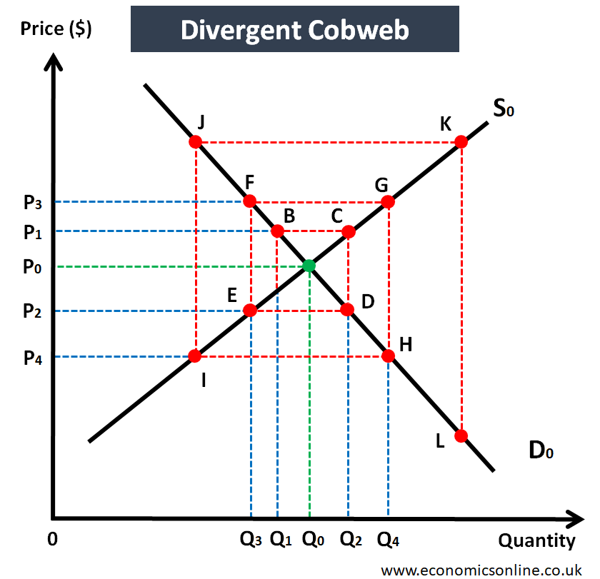
In the above diagram, the equilibrium price is P0 and the equilibrium quantity is Q0.
- Suppose that due to bad weather, the quantity supplied is at Q1. At Q1, buyers are willing to pay a higher price of P1 as shown by point B and sellers sell their quantity at this price.
- Next year, the farmers base their production decision on last year’s high price of P1 and increase their supply to Q2 as shown by point C.
- At Q2, buyers are willing to pay a low price of P2 as shown by point D.
- Next year, they consider this low price P2 and produce Q3 quantity at point E.
- At Q3, they get a high price of P3 as shown by point F.
- Next year, due to the high price of P3, they produce at Q4 as shown by point G, which leads to a low price of P4 as shown by point H and the cycle continues.
Since the price is gradually diverging away from P0, this diagram illustrates a divergent cobweb in which price fluctuations are increased. This cobweb is less common in real life.
Limitations of Cobweb Theory
The following points explain some limitations of cobweb theory:
Rational Price Expectations
It is a limitation of the cobweb theory because farmers predict the supply of their product entirely based on the previous year’s supply and also assume that it will be the same next year. But this assumption does not work in the real world. Farmers can see if it is a good year or a bad year and can understand the price changes with time.
Switching Supply
It is also a limitation of cobweb theory, as switching the supply is not an easy task. For example, a potato grower can only grow potatoes expertly. It is not easy for him to give up farming potatoes and start growing wheat.
Other Factors
In real life, there are many other factors which farmers consider while making the production decisions and price is just one factor. Other factors may include coast of seeds and fertilizers, labour cost, taxes and subsidies, weather conditions and the prices of other crops etc.
Buffer Stock Schemes
The main limitation of this concept is that governments use buffer stock schemes in which the government and other producers tie up together to limit price changes by buying surplus.
Conclusion
In conclusion, the cobweb theory is related to the agriculture commodity markets and explains the cyclical changes in the prices of wheat and other agriculture products from one season to the other. In this theory, the present events totally depend on the previous happenings. This theory explains that the farmers plan the production of their agricultural based on the previous prices, but in the real-world, price fluctuations may occur that are not always in their favour.

