
Competitive labour markets
Competitive labour markets
The demand for labour – marginal productivity
The demand for factors of production is derived from the demand for the products these factors make. For example, if mobile phones are in greater demand, then the demand for workers in the mobile phone industry will increase, ceteris paribus.
The demand for labour will vary inversely with the wage rate. To understand this we need to consider the law of diminishing returns. This states that if a firm employs more of a variable factor, such as labour, assuming one factor remains fixed, the additional return to extra workers will begin to diminish. To explore this process, we need to consider the total physical product (output) produced by a series of workers, which will enable us to measure the individual output from each additional worker – the marginal physical product (MPP).
Consider the following data for a small firm producing handmade wax candles.
| Workers | Total physical product | Marginal physical product |
| 1 | 1000 | |
| 2 | 1900 | 900 |
| 3 | 2700 | 800 |
| 4 | 3400 | 700 |
| 5 | 4000 | 600 |
| 6 | 4500 | 500 |
| 7 | 4900 | 400 |
| 8 | 5200 | 300 |
Demand is based on the value to the firm of the marginal physical product produced by each worker. For example, if candles are £2 each, the firm can calculate the revenue derived from each worker’s physical output. The value of the extra output is called marginal revenue product (MRP), and this is calculated by multiplying MPP and price, as follows:
| Workers | Total physical product | Marginal physical product | Marginal revenue product |
| 1 | 1000 | ||
| 2 | 1900 | 900 | 1800 |
| 3 | 2700 | 800 | 1600 |
| 4 | 3400 | 700 | 1400 |
| 5 | 4000 | 600 | 1200 |
| 6 | 4500 | 500 | 1000 |
| 7 | 4900 | 400 | 800 |
| 8 | 5200 | 300 | 600 |
Deriving a demand curve
We can now find the number of workers that would be employed by a profit maximising firm at various wage rates. The profit maximising firm will employ workers up the point where the marginal benefit, in terms of the MRP, equals the marginal cost of labour (MCL), which in this case is the wage rate (W).
For example, at a wage rate of £1,200, the firm will employ 5 workers, because at 5 workers, MRP = MCL. At a lower wage of £800, the firm will employ 7 workers, and so on. This means that a demand curve can be derived. In labour market theory, the demand for labour is identified as MRP=D.

The supply curve of labour in a competitive market
In a perfectly competitive labour market, where the wage rate is determined in the industry, rather than by the individual firm, each firm is a wage taker. This means that the actual equilibrium wage will be set in the market, and the supply of labour to the individual firm is perfectly elastic at the market rate.
Equilibrium wage in the labour market, and supply for the individual firm.

The simple model of market wage
The competitive market wage rate, and the quantity of labour employed, is determined by the interaction of demand and supply. The equilibrium wage rate is the rate that equates demand and supply, as illustrated below.
Equilibrium wage rate
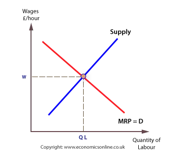
Labour supply for the whole market is assumed to be positively related to the wage rate, and the market supply curve slopes upwards.
Changes in market wage
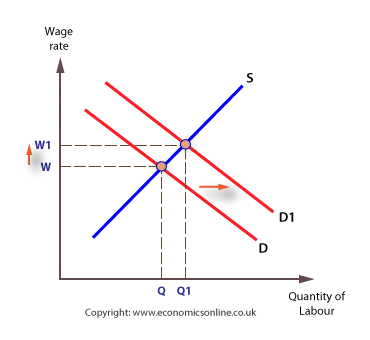
Market wage may change following a change in an underlying condition of demand or supply.
Demand can change, and the demand curve will shift, under a number of circumstances, including changes in:
- The productivity of labour.
- The price of the product.
- Demand for the product.
Shifts in the demand for labour
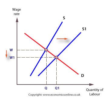
Labour supply can change under a number of circumstances, including changes in:
- The length of the working week.
- Participation rates.
- Demographic factors, such as migration, and changes in the age structure of the population.
- Qualifications and skills required.
- The length of training.
Shifts in the supply curve
See: monopsonists